Showcase: ETOPO over the central Andes
A real-data companion to the idealised tutorial. Where the tutorial recovers a synthetic spectrum whose answer is known a priori, this example runs the full CSA pipeline on a real ICON grid cell over the central Andes near Aconcagua (~32°S) — a strong orographic gravity-wave source with dramatic coast-to-summit relief (Pacific shelf to ~4.4 km summits in a single cell).
It ships with everything it needs (examples/data/etopo_andes/ is ~130 KB: a
single-cell ICON grid subset plus a coarse-grained ETOPO slice), so a reviewer
or new user can clone and run it in a few seconds — no data download.
Run it
After pip install -e .:
python examples/icon_etopo_andes.py
It prints the top mode amplitudes and the spectrum shape, then writes a
three-panel diagnostic figure to examples/output/icon_etopo_andes.png. The
numerics are computed live (not pinned), so they will differ slightly across
LAPACK builds — this script is for human inspection, not regression gating.
What this adds over the idealised tutorial
The CSA algorithm is identical to the tutorial (first approximation → top-N
mode selection → constrained second approximation via
pycsa.wrappers.interface.get_pmf). What’s new here is everything
around it — the parts that make it a real, production-shaped run:
Real ETOPO topography loaded through the production loader
pycsa.core.io.ncdata.read_etopo_topo()— the same data path the global HPC pipeline uses, including the bounding-tile assembly across the two bundled ETOPO slices.Ocean-aware masking. ETOPO carries bathymetry, so the cell spans sea floor to summit. The example clamps deep bathymetry to −500 m for the spectral fit, then excludes ocean below −200 m from the analysis mask — the atmosphere “sees” the sea surface, not the seafloor. In the figure, deep ocean and the cell exterior render white; the shallow shelf (−200…0 m) stays blue. This mirrors
runs/icon_etopo_global.pyexactly.The production diagnostic plot. The figure is rendered by
pycsa.plotting.diagnostics.plot_cell_diagnostics()— the same routine the global run emits per cell, with the same ocean-aware colormap. So the figure below is representative of what a global run produces for any land cell.
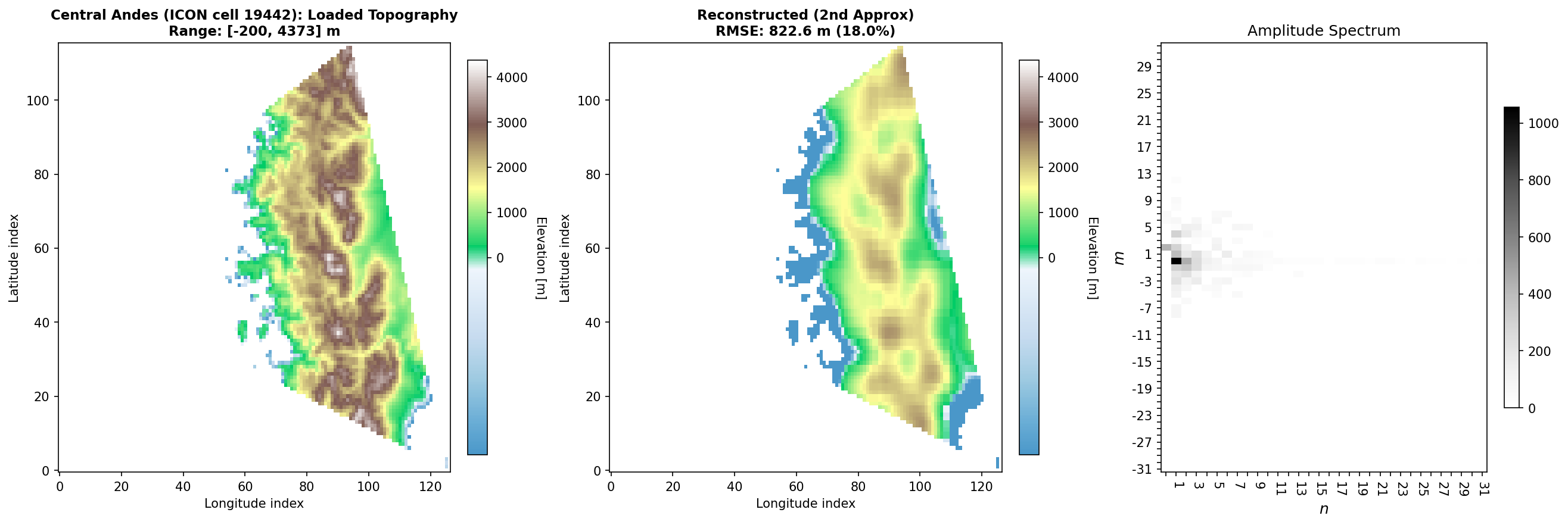
Fig. 3 Left: the loaded ETOPO topography for the cell (ocean-aware colormap;
shelf in blue, summits in brown). Middle: the CSA second-approximation
reconstruction from the selected modes, with its RMSE. Right: the amplitude
spectrum on the n × m (64 × 32) wavenumber grid — a sparse set of
modes carries most of the energy, which is the whole point of the
constrained approximation.
Where this fits
This is one cell of what HPC reproducibility guide runs over all 20,480
cells of the ICON R02B04 grid — same ETOPO loader, same ocean masking, same
per-cell diagnostic plot, just wrapped in Dask memory-batching and a worker-local
tile cache (pycsa.compute.context.ComputeContext). If you want to see
the method scale up, that page is the next step.
The two hardest “corner” cells — a false-positive-dateline cell and a south-pole
cell — are pinned by the reproducibility suite at tests/reproducibility/ and
gated in CI; the numerics here are deliberately left live for inspection.